Most of the time, when you create a chart, you can leave the Range selection for the X- and Y-axes on “Auto”. Recent versions of Qlik Sense have improved the logic that’s used to determine these ranges and it’s also usually the most efficient option in terms of refresh time—and your time. But there are times when your requirements or your data characteristic don’t fit the standard logic that the visualization engine uses to determine the ranges for axes on a chart. In these cases, you’ll need to customize how the scale for the X-axis or Y-axis; or both, by using a custom formula.
So, what situations require us use a custom formula for an axis? Custom Min/Max values are most often set for the Y-axis, either when the choices for this range are not obvious or when you’re using reference lines. This post focuses on the latter case.
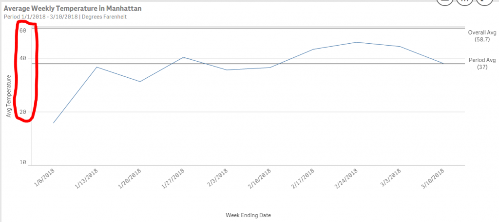
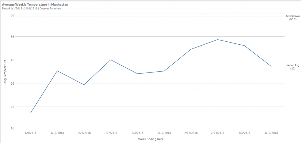
The chart below shows the average weekly temperature in Manhattan in 2018. I’ve added two reference lines—one showing the overall average temperature (for all the data) and one showing the average temperature for the period shown (filters applied). Since I haven’t filtered anything yet, both are the same. So far, so good.
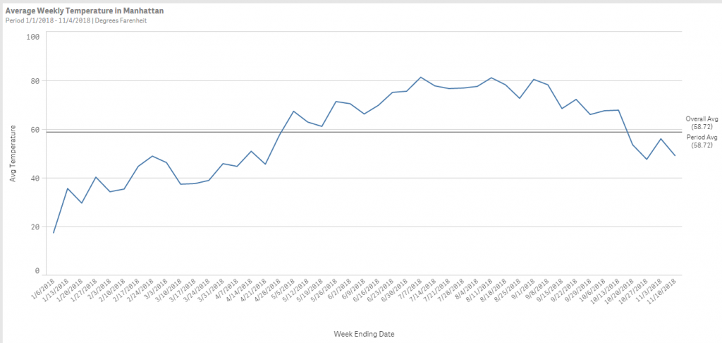
I’ll list the formulas used for the dimensions and measures for clarity and because I’ll refer to them later.
Dimension: [Week Ending Date]
Measure: [Weekly Temperature]
Reference Line for Overall Avg: Avg({1} [Weekly Temperature])
Reference Line for Period Avg: Avg([Weekly Temperature])
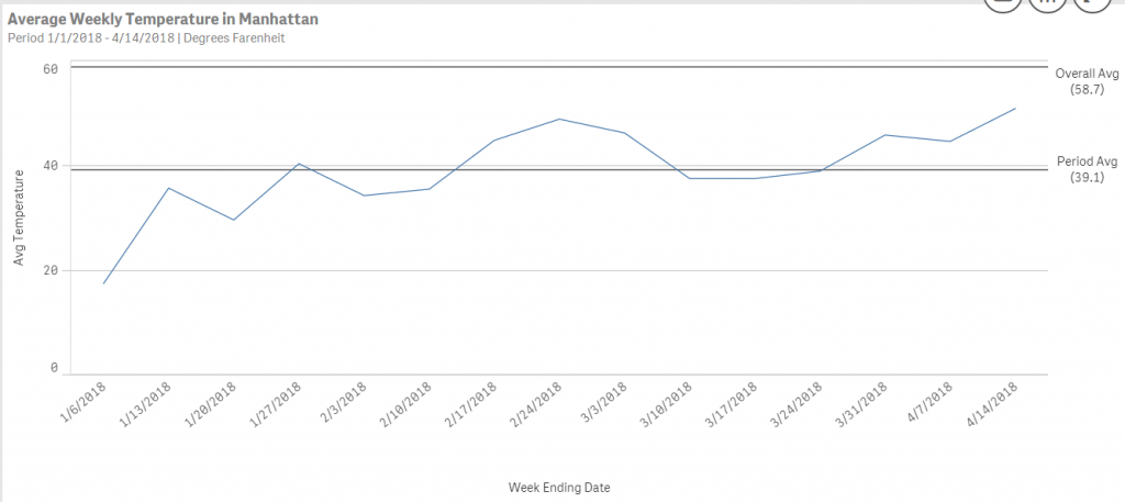
Here’s another example when I’ve selected a subset of the dates. Now we have different values for the two reference lines and the chart still renders the way we’d expect. Still good.
The issue discussed in this post appears when I select a subset of the dates that causes the measures (the lines) that are displayed to be far from one or more of the reference lines. In this case the chart optimized the display for the normal range, but doesn’t show the reference lines that fall way outside the range. Instead, it shows a small icon at the upper or lower right corner of the chart, depending upon the line that isn’t shown.
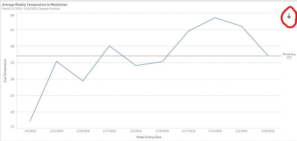
Let’s look at how the chart uses our data to create the Y-axis values when we choose the “Auto” setting—It’s using the values of the data in the measures, but not the values for the reference lines This makes sense—the display favors the main chart data—but if the reference lines are also important then using “Auto” is probably not the best option.
There are two approaches to handling this solution. Both have a different visual result.
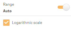
The first approach is the quickest and easiest. Simply click the checkbox for “Logarithmic scale” that’s just below the “Range” selector.
Qlik Sense will always adjust the Y-axis to include the full range. That’s good, but the values on the axis will not be evenly distributed and though the lines shown will be scaled to those values, the shape of the lines may not be as expected. You can see this effect in the sample below.
This could be confusing to users—especially when the visual presentation of the curve (or trend) is important. In this case, there is another approach that will solve this issue. It requires that we explicitly set the formula that the engine will use to calculate the scale and values for the axis.
First, let’s look at the result (below). Compare it to the example above. Both are correct, but the second one presents a much more natural-looking curve and a Y-axis with evenly-spaced values. This is closer to what a user would expect.
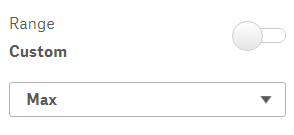
Here’s how to accomplish this. First, toggle the “Range” selector to “custom”. This will allow us to select a custom formula for the “Min”, “Max”, or both. In this example, I’ve selected the “Max”. I’ll let Qlik Sense set the “Min” automatically.
Then, enter the formula to use for the “Max” value. I’ve shown the one used on this chart.
=Ceil(
RangeMax(
Max(Aggr(Avg([Weekly Temperature]), [Week Ending Date])),
Avg({1} [Weekly Temperature]),
Avg([Weekly Temperature])
), 10)
Let’s take a look at a generic version of the formula used.
=Ceil(
RangeMax(
Max(Aggr(the measure on the chart, the dimension for the X-axis)),
the formula used for the first reference line,
the formula used for the second reference line
), 10)
The formula takes the highest value of the measure (Y-value) on the chart
Max(Aggr(the measure on the chart, the dimension for the X-axis))
Then it takes the maximum value (RangeMax) of that, or any of the reference line formulas
RangeMax(
Max(Aggr(the measure on the chart, the dimension for the X-axis)),
the formula used for the first reference line,
the formula used for the second reference line
)
And finally, it rounds that up to the nears increment of 10, using the Ceil function. You can change that increment depending upon the increment you’d like for the upper value, or if you’re using a percent scale.
The advantage of the second approach is that you ensure that all of the reference lines appear on the chart and that the Y-axis and the lines are normally proportioned on the chart.
Which approach is best? It really depends upon your requirements, your data and what the expectations of your users will be. Try this on your charts. You will probably find situations where your dataset is so large that using custom axis values is inefficient. That might be a limiting factor, or it might mean that you need to optimize your data model—but that’s a topic for another post.
If you need examples of how to scale the “Min” value, or how to do this for an axis that shows a percent please post in the comments.